Computer Vision Introduction
Introduction
General Definition: Computer Vision uses light information (ie. pictures, infared scan, etc) into meaning (ie. geometric model, natural language).
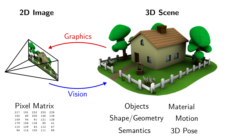
Relation with Computer Graphics
Computer graphics is the inverse process of computer vision:
- For computer graphics, we are given the 3D scene, for example the object model, the camera pose, and material information, and we render the corresponding 2D image.
- For computer vision, we are only given the 2D image(s), and we need to extract information from such limited information.
Why is Computer Vision Hard?
Many different 3D scenes can yield the same 2D image. Therefore additional constraint/assumptions about the scene is required.
Image Formation
Homogeneous Vector (2D)
A 2D point can be written in inhomogeneous coordinates as:
\[\mathbb x = \begin{pmatrix}x\\y\end{pmatrix}\]The homogeneous representaion (also known as Real Projective Space in mathematics) is
\[\tilde{\mathbb x} = \begin{pmatrix} \tilde x\\\tilde y\\ \tilde w\end{pmatrix} = \begin{pmatrix} x\\y\\1\end{pmatrix}\]With two vectors $\mathbf{x,v}$ equal in homogeneous space iff $\mathbf x = \lambda \mathbf v$. The point with $\tilde w = 0$ is defined as the point at infinity.
The 2D line can be expressed using $\tilde I = (a,b,c)^T$, with
\[\{\bar{\mathbf x} | \tilde I^T \bar{\mathbf x} = 0\}\]The line at infinity is defined as $\tilde {I}_\infty = (0,0,1)^T$.
Cross product can be described as a multiplication of a skey symmetric matric multiplied by a vector. Line joinning two points $\bar{\mathbf x}_1 = \bar{\mathbf x}_2$ can be compactly written as:
\[\tilde{I} = \bar{\mathbf x}_1\times \bar{\mathbf x}_2\]The intersection of two lines is the point $\tilde{I}_1\times \tilde{I}_2$, and such a point can be the point at infinity.
2D Conics is defined using the equation:
\[\{\tilde {\mathbf x} | \tilde {\mathbf x}^T \mathbf Q \tilde{\mathbf x}\}\]Homogeneous Vector (3D)
We can simply extend the 2D vector by adding a $z$.
\[\tilde{\mathbb x} = \begin{pmatrix} \tilde x\\\tilde y\\\tilde z\\ \tilde w\end{pmatrix} = \begin{pmatrix} x\\y\\z\\1\end{pmatrix}\]